Musings from Carbon’s Engineers

Fast Inside-Outside Segmentation

By Nicholas Harrington, September 9, 2021
Credits: Nicholas Burgess, Kesavan Kushalnagar, James Clark, John Walker

This post will detail a robust algorithm for inside-outside segmentation of points when provided a boundary representation of a solid. To put it another way, we are given the surface of a solid and we would like to know which points are inside the solid and which points are outside the solid. We have the orange peel and need to extrapolate the rest of the orange. This problem is of particular importance for Carbon 3D printers. Our printers, which use the Carbon Digital Light Synthesis™ (Carbon DLS™) 3D printing process, operate in voxel space. The most common model formats for 3D printing provide a boundary representation, usually a triangle mesh.

The algorithm we will detail works in arbitrary dimensions, though anything more than three dimensions makes my brain hurt. Because of the nature of our existence, it has the most practical applications in three dimensions. The algorithm is a bit easier to illustrate in two dimensions, however. For this post, I will focus on a 2D version of the algorithm.

In the 2D case, we have a list of directed line segments, and we need to determine which points on the 2D plane are inside the shape defined by the line segments.

The first issue we run into is that our problem statement is poorly constructed for any surfaces that do not form a watertight object. If there are gaps in the surface, we cannot definitively say if a point is inside the object or not. This is a deeply frustrating aspect to this problem. We rely on our ability to convert a boundary representation of a solid to a voxel representation to print. Any defects in the surface description of the model force us to guess which points are inside the shape.

To illustrate this issue, let’s work through a simple example. If we are given a closed outline of a shape, we can easily fill in the shape:

But let’s say we are missing a section of the shape:

Around the gap we are just guessing. We could legitimately choose the set of purple points as being inside the shape. We could also legitimately choose the cyan points. Both are valid.

At this point, we can either throw our hands into the air and bemoan that we live in a world where so many important things are unknowable, or we can reframe the problem we are trying to solve.

Instead of trying to solve a particular problem, we just want to find an algorithm that has the following set of properties:

1. If all the surfaces are closed, meaning we can know with 100% certainty if a point is inside or outside the shape, we need to correctly identify the points inside and outside the shape.
2. If we introduce a defect, the size of the region that changes its inside/outside determination should be proportional to the size of the defect. So if you introduce a small defect, only a small region of space should flip from inside to outside, or vice versa.
3. We should know when we are guessing. If there are points with an ambiguous inside/outside state, we should be able to identify those points.

Fortunately, there is an existing published example of an algorithm that does just this. There is a great  paper^[1] that computes the winding number to determine if a point is inside a shape or not. In two dimensions, the winding number of a point is the number of times a point is surrounded by the outline of the shape going counterclockwise. A winding number of one means that the point is encircled one time by a curve going counterclockwise. A winding number of negative two means that the point is surrounded by two loops going clockwise. One can generalize the concept of winding number to include fractional numbers. If a point is partially enclosed by a loop, we can write down how fractionally surrounded it is. Below are some examples of winding number estimates for points.

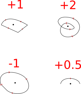
While the paper does something a bit more complicated, for conceptual simplicity, we can say a point is inside our shape if the winding number is 0.5 or greater at that location. This gives us an algorithm for determining if a point is inside or outside a shape. We compute the winding number at all the locations we care about. We then say any points with a winding number above our 0.5 threshold are inside the shape.

We can see that this meets our three criteria. If all the surfaces are watertight, all of the  computed winding numbers will have integer values. Anything with a winding number of one or higher is definitely inside the shape. If defects are introduced, the winding number for nearby points are the only ones that are largely affected by the defect. And, the computed winding number will only be a non-integer value if we are guessing. That’s one, two, and three right there.

This is not the algorithm we use, however. The big problem with this algorithm is that it is relatively slow. For L line segments and P points, the worst case runtime is O(LP). The original paper and a separate paper^[2] suggest ways of improving the runtime. These fast winding number methods do a great job of improving the runtime, but it still is too slow for our purposes. The authors of the fast winding number paper included an implementation with the IGL library.  Running the fast winding number algorithm with our density of voxels and mesh complexity can take multiple hours.

Carbon 3D printers often print models with billions of voxels. The triangle meshes that are voxelized can have tens to hundreds of millions of triangles. We want to be able to slice a project in a couple minutes. Slicing is just 3D printing slang for converting from the surface representation to the voxel representation. Because of our strict timing constraints, we are limited in the operations we can run. Just calling a sine function a billion times takes about a minute on the computer I’m using to type this.

Computing the winding number is too slow for our uses, but the idea behind the algorithm is fantastic. The authors reframed the problem of inside/outside segmentation to be entirely in terms of computing something well defined that has the three properties we want from an algorithm. We just need to find a problem that we can compute more efficiently.

Let’s convert the inside/outside segmentation problem to a heat problem. We will say that there is a one degree temperature difference at the surface of the model. A point just inside the surface of the model will be one degree hotter than the point just outside the model. This is just a delta in temperature. We could also say that a point just outside the model is one degree cooler than a point just inside the model. All other points are in thermal equilibrium. Outside the region of interest, we will set the temperature to 0. We use that as our Dirichlet boundary condition. After we solve for the temperature everywhere, we will just say that points with a temperature/insideness over 0.5 are inside.

If we restrict ourselves to only points on a regular grid, the heat equation can be solved in linear time, O(P), or log-linear time O(P log(P)). Since we are solving this problem for Carbon 3D printers, and they only care about points on a regular grid, the idea of using the heat equation is promising from a runtime perspective.

Even before we work through the math, we can see how this should meet our three criteria. If all the surfaces are closed, the temperature inside our shape should be a positive integer value. Small changes in the surface mesh should only have a small effect on the temperature in the region. And for number three, if we see non-integer values of temperature, we know we are guessing.

For those that don’t sleep with a statistical physics book under their pillow, the heat equation has the form:

T is the temperature/insideness that we are solving for. f is the source term. It encapsulates the temperature change at the boundary of the shape. For all points not within one grid spacing of the edge, f is set to 0. The Laplacian operator in this equation is the discrete Laplacian operator. The equation we listed above is often referred to as the Poisson equation. We are not going to go into the details of solving it. It is an extremely well studied equation and there are lots of resources available that detail methods for solving it. We in particular are just using the canned Poisson solver that Intel provides as part of the MKL library.

If you have never had the pleasure of learning about the Laplacian operator, , don’t panic. All the operator does is take the difference between the point we are at and the average of all of its neighbors. It’s why a system in thermal equilibrium satisfies the equation:

The temperature doesn’t change if at every point the temperature is the same as the average of its neighbors. Hopefully that makes intuitive sense.

To be explicit, the discrete Laplacian operator we are using has the form:

The delta x in the equation is our grid spacing. Our goal is to take the edge information of our shape/solid and convert it into an estimate for our source term, f. If we are talking about one solid/shape that does not self intersect, we could just compute the signed distance function locally, within one grid spacing of the boundary, and then convert this signed distance function (SDF) into our source term, f. The signed distance function at a point is the distance from that point to the nearest surface of a solid. The sign is positive inside the shape and negative outside, though that convention is often flipped. Using the form of the equation above, one can convert between the SDF to an estimate for the discrete Laplacian applied to our filled in shape.

This whole process seems kind of circular. If we know the SDF why bother with the rest of the process? Estimating the SDF in all of space is a computationally expensive operation. We are only estimating the SDF within one grid spacing of the surface of the part. We only need to estimate the SDF in this region because it is the only region that will have a non-zero f value. If there are gaps in the surface of the solid, we rely on finding our temperature field to fill them in. The soul of this procedure is similar to the technique described in a conference proceeding from the early 2000s^[3].

Self intersecting models or multiple overlapping solids throw a spanner in the works though. The procedure of estimating the signed distance function and then converting it to the estimate for the Laplacian erases the contribution of overlapping edges. If a model has two surfaces in the same pixel, the SDF we estimate just stores the distance to the nearest surface. It has no knowledge that two surfaces are contributing to the estimate. Ideally we would add the contribution from each surface to the estimate of the Laplacian of the filled-in shape. I wish I had a more clever solution to this problem, but to get around it we just preprocess the solid/shape and divide it into different solids and self intersecting sections. The process of dividing it is currently done by finding connected sections of the surface mesh and also looking for self intersections. It exposes the whole procedure to possible misclassification errors. Even with misclassified models, the results are usually still good. It’s just a bit ugly from a theoretical side. If you know a better way to estimate a surface’s contribution to our source term, f, let me know.

Writing it all out, the procedure is:

1. Take the input surface and divide it into separate solids. If there are self intersecting sections, divide those into separate solids.
2. For each solid:
   1. Estimate the SDF of the solid
   2. Convert the SDF to an estimate of what the discrete Laplacian operator applied to the solid would be, f
   3. Add the individual solid’s source term, f, to a collective source term, f_sum
3. Solve the Poisson equation using f_sum as the source term for T.
4. Threshold T. All points above 0.5 are inside the shapes.

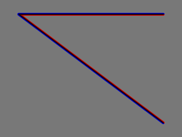
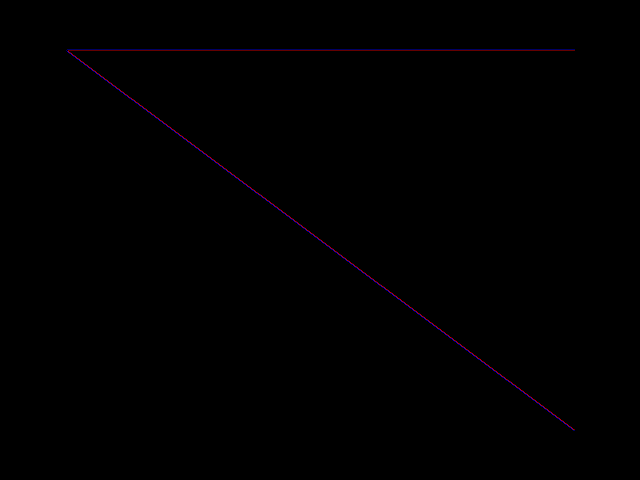
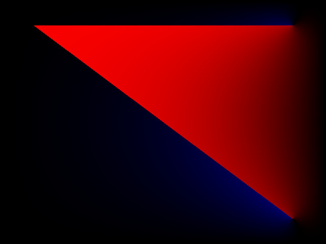
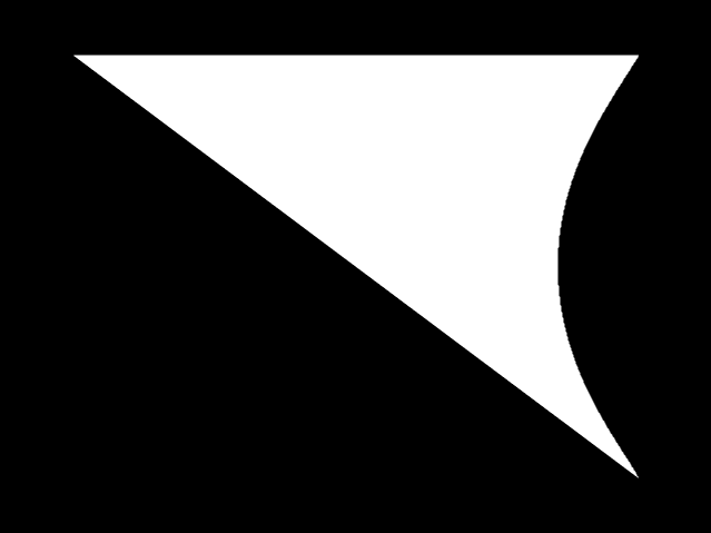
Let’s look at some 2D examples for the procedure. First let’s see how two thirds of a triangle works with this procedure:

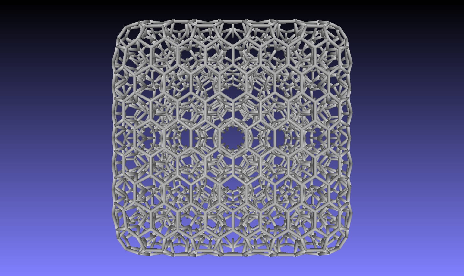
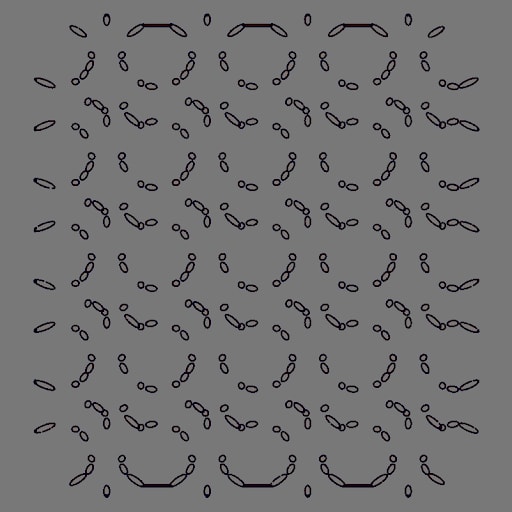
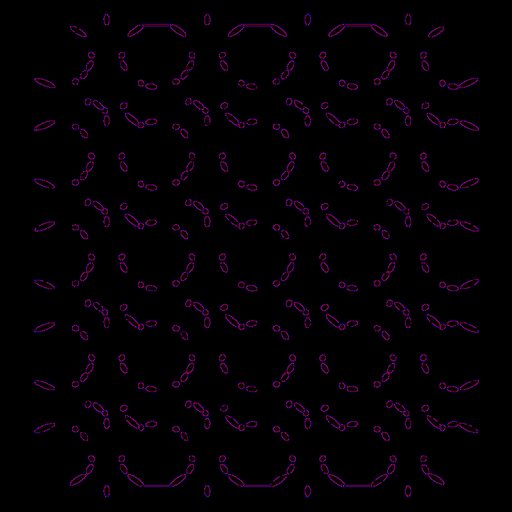
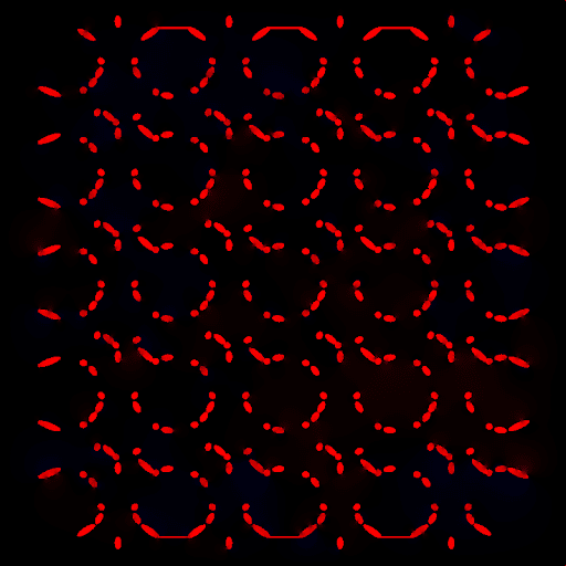
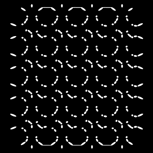
Now let’s look at a single slice of a strut based lattice that I deleted five percent of the surface from.  Just for reference, the part before the deletion looks like:

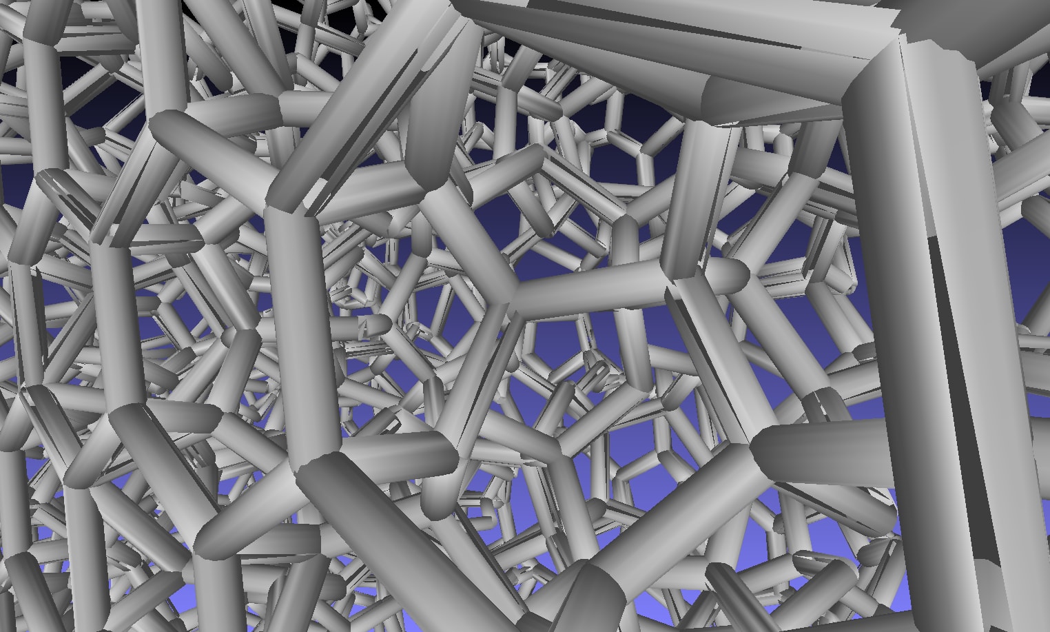
And here is a close up after 5% of the triangles were deleted:

With our implementation, the runtime for R triangles and P points is O(R lg(R) + P lg(P)). The preprocessing to divide the shapes takes R lg(R) time. Solving the Poisson equation takes P lg(P) time when using FFT based methods. Solving the Poisson equation can be done in linear time using multi-grid methods. The log-linear time of Intel’s solver is an extremely fast log-linear time, however. If you can assume no self intersections, the triangle processing time can be made linear quite easily.

Since the winding number based methods are the state of the art, let’s compare the Heat equation based method to those techniques. The runtime of our method is much faster asymptotically and practically. For a model with four million triangles run on one billion voxels, the IGL implementation of the fast winding number algorithm takes 2,700 CPU minutes. The Heat equation based method takes about 20 CPU minutes. It only works on a regular grid of points, and there is the awkwardness of attempting to classify which solid the triangles belong to before performing the operation. We trade a bit of theoretical niceness for a massive improvement in runtime.

3D as It’s Meant to Be

Interested in utilizing Carbon to accelerate product development? Reach out to us at sales@carbon3d.com to learn more!